library(tidybayes)
library(bayesplot)
library(brms)
library(tidyverse)

df <- tribble(
    ~date, ~dislocations, ~tape, ~hours,
    1, 5, 0, 12,
    2, 4, 0, 12,
    3, 3, 0, 12,
    4, 1, 1, 12,
    5, 0, 1, 12,
    6, 1, 0, 12,
    7, 3, 0, 12,
    8, 2, 0, 12,
    9, 0, 1, 12,
    10, 1, 1, 8,
    10, 1, 0, 4,
    11, 0, 1, 12,
    12, 1, 1, 12,
    13, 1, 0, 2,
    13, 2, 1, 10
  ) |>
  mutate(
    across(.cols = everything(), .fns = as.integer),
    day = hours / 12
)In the last couple of years, my girlfriend sprained her ankle multiple times. A month ago, a ligament in her ankle began frequently slipping out of place. She has to locate it back manually, a couple of times per day. Ouch.
She decided to try Kinesio tape to improve her condition. Since she sometimes forgets to put it on, this provides an opportunity to evaluate if using the tape reduces the daily number of dislocations.
We will use Bayesian Poisson regression to tackle the problem. Why Poisson?
If the number of trials
nis very large (and usually unknown) and the probability of a successpis very small, then a binomial distribution converges to a Poisson distribution with an expected rate of events per unit time of \(\lambda = np\). - Statistical Rethinking by Richard McElreath
So, during the day, there are a lot of opportunities (trials) for dislocations, but dislocations (successes) happen rarely.
Data
Here’s the data I collected:
The data represents dislocation counts per date (the actual date is not important so it’s just an integer). I assumed there are twelve active hours per date. Because sometimes she used the tape for a couple of hours, there can be multiple rows per date with the number of hours that sum up to twelve. Dummy variable tape denotes whether she used the tape. Based on the hours I calculated the portion of the day.
From the plot below we can see there’s no trend in the number of dislocations.
df |>
  mutate(dislocations_per_day = dislocations / day) |>
  ggplot(aes(date, dislocations_per_day, color = as.factor(tape))) +
  geom_point() +
  labs(title = "Dislocations per date seem stable", color = "Tape use")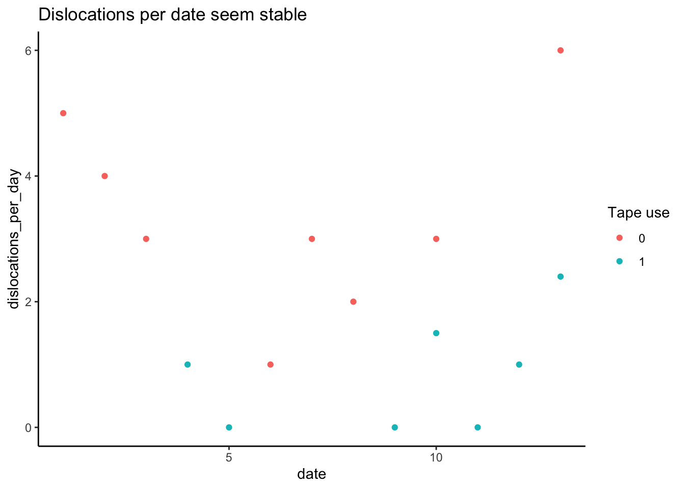
Modeling
Our assumptions:
- she uses the tape randomly1 and doesn’t change her behavior once she wears it;
- the dislocations are independent of one another;
- the average rate at which events occur is constant.
There’s no placebo in our experiment, so a placebo might account for potential improvements. However, there are no side effects of using the tape (besides monetary) so we are fine even if the improvement would be due to placebo.
The system can be described using the following formulas:
\[ dislocations_i \sim Poisson(\lambda_i) \] \[ log(\lambda_i) = log(day_i) + a + b * tape_i \] \[ a \sim \mathcal{N}(0.5, 1) \] \[ b \sim \mathcal{N}(0,1) \]
Daily \(dislocations\) follow the Poisson distribution with parameter \(\lambda\). \(log(\lambda)\) is calculated as a linear combination of log(day) that presents a duration, parameter a, rate of dislocations without the tape, and parameter b that represents the change in dislocation rate associated with using the tape. Since we have number of dislocations per different time durations, not only per day, we include the \(log(day_i)\) term. This makes sense because we are interested in the rate of dislocations per day (represented by twelve active hours):
\[\frac{\lambda_i}{day_i}=exp(a + b * tape_i)\] If we \(log\) and apply \(log(a/b) = log(a) - log(b)\) on both sides, we get:
\[log(\lambda_i) - log(day_i) = a + b*tape_i\] Now we only need to move \(-log(day_i)\) to the right side. Voila!
To implement these formulas in R, we’ll use the brms package. In brms syntax, our intercept parameter \(a\) is represented by Intercept, while our tape effect parameter \(b\) is represented by tape.
d <- transmute(df, tape, dislocations, day)

m <- brm(
  formula = dislocations ~ offset(log(day)) + tape,
  family = poisson(),
  prior = c(
    prior(normal(0.5, 1), class = "Intercept"),
    prior(normal(0, 1), class = "b", coef = "tape")
  ),
  data = d,
  warmup = 200,
  chains = 4,
  cores = 4,
)
We’ll also calculate the ratio between dislocation rates of taped and non-taped ankle.
posterior_samples <- as_draws_df(m) |>
  mutate(ratio = exp(b_Intercept + b_tape) / exp(b_Intercept))
By calling summary we can see that tape has a negative value, denoting that the tape helps.
summary(m) Family: poisson
Links: mu = log
Formula: dislocations ~ offset(log(day)) + tape
Data: d (Number of observations: 15)
Draws: 4 chains, each with iter = 2000; warmup = 200; thin = 1;
total post-warmup draws = 7200
Regression Coefficients:
Estimate Est.Error l-95% CI u-95% CI Rhat Bulk_ESS Tail_ESS
Intercept 1.04 0.23 0.57 1.46 1.00 6134 4818
tape -1.16 0.43 -2.03 -0.35 1.00 3203 4096
Draws were sampled using sampling(NUTS). For each parameter, Bulk_ESS
and Tail_ESS are effective sample size measures, and Rhat is the potential
scale reduction factor on split chains (at convergence, Rhat = 1).We would have to exponentiate the values of Intercept and tape to get the actual dislocation rates. Below, we’ll plot the posterior distribution of ratio that is calculated as \[ratio = \frac{e^{Intercept+tape}}{e^{Intercept}}=\frac{\lambda_{tape}}{\lambda_{no tape}}\]
ggplot(posterior_samples, aes(ratio, fill = after_stat(abs(x) < 0.5))) +
  stat_halfeye() +
  labs(title = "Dislocation rate decreases to one third when using the tape")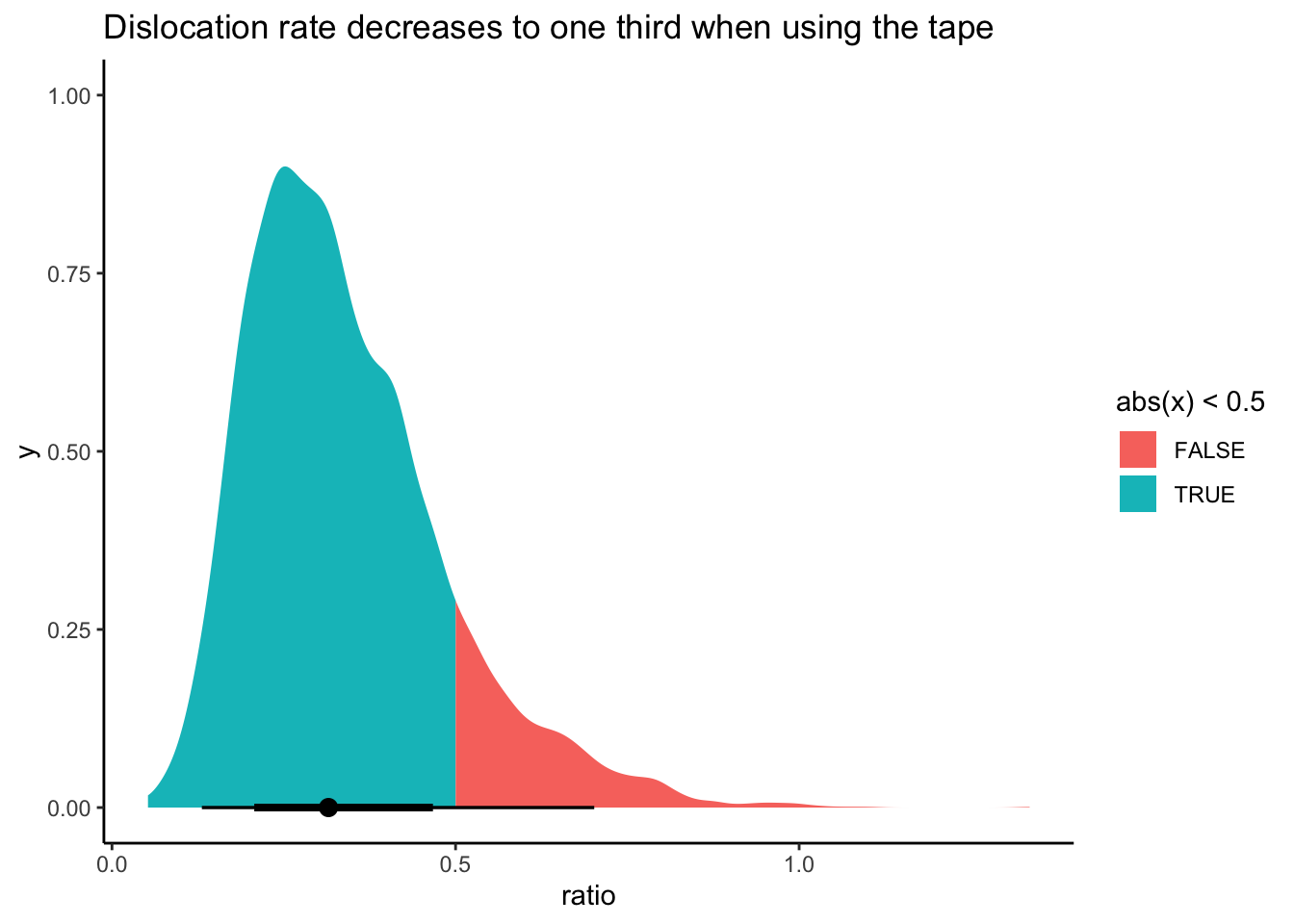
Bayesian approach enables us is to make probability statements about the posterior distributions. For example, we can calculate probability that ratio is lower than 0.5 (integral of blue area on the plot above):
summarise(posterior_samples, prob_less_than_0.5 = mean(ratio < 0.5))# A tibble: 1 × 1
prob_less_than_0.5
<dbl>
1 0.869Let’s also do a posterior predictive check - simulating replicated data under the fitted model and comparing these to the observed data2. This tells us whether the model gives “valid” predictions about reality.
pp_check(m, type = "dens_overlay_grouped", group = "tape", ndraws = 50) +
  labs(title = "Comparison of empirical data distributions")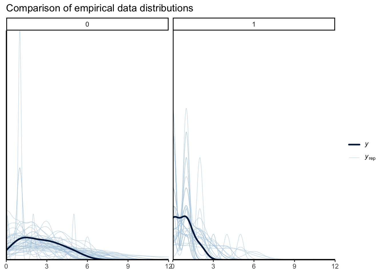
We can see that true data has shorter tails compared to the simulated ones. To account for overdispersion, we could use negative binomial model, which assumes that each Poisson count observation has its own rate.
From now on, she uses Kinesio tape every day. I’m kidding. Writing this blog post took me so long that her condition improved by itself. Time works even better than Kinesio tape.
Footnotes
She could flip a coin in the morning and wear a tape based on the outcome.↩︎