The bootstrap is a resampling method that makes it easy to compute the distribution of any statistical estimate. Its main downside is computational power that makes it difficult to perform it on big data.

When reading An Introduction to the Poisson bootstrap from The Unofficial Google Data Science Blog¹, I came across the bootstrap approximation that bypasses the big data problems and it’s even easier to implement. The approach uses frequencies from Poisson distribution to model the number of occurrences of each observation in the resample.

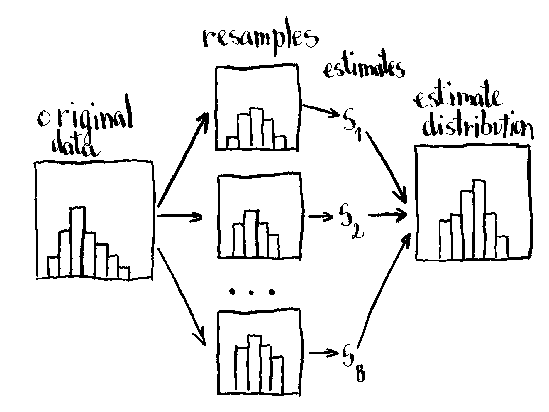
Bootstrap procedure is the same in the classical and Poisson version. The difference lies in the calculation of resamples.

The classical non-parametric bootstrap

The classical bootstrap is obtained by collecting random observations with replacement from the original sample. These collections, also called resamples, are the same size as the original sample. On each resample we calculate an estimate for the statistic of interest. This procedure is repeated over and over again (order of hundreds or thousands) so we obtain the distribution of the statistic. In case our statistic of interest is the mean, we can use this function to obtain the resample and calculate the mean:

classical_boot_mean_estimate <- function(x) {
  mean(sample(x, length(x), replace = TRUE))
}

The Poisson bootstrap

We can also look at the bootstrap as assigning the number of occurrences for each observation in any given resample as \(Binomial(n, \frac{1}{n})\)². Since the total number of observations in each resample is constrained by n, the counts are jointly \(Multinomial(n, \frac{1}{n}, ..., \frac{1}{n})\). This means the counts are negatively correlated with one another. It turns out that for estimators involving rations of sums, we could sample from \(Binomial(n, \frac{1}{n})\) and do fine for samples with more than 100 observations. We can even use

\[\lim_{n \to \infty} Binomial(n, \frac{1}{n}) = Poisson(1)\]

that allows us that we don’t need to know the number of observations in advance and other computational benefits (see Google’s (unofficial) blog post and publication for more on this topic).

To repeat, with the equation presented above we can calculate the mean of the resample with the equation:

\[\bar{x}*=\frac{\sum x_i \times p_i}{\sum p_i}\]

where \(\bar{x}*\) presents the mean of the resample, \(x_i\) observations in our original sample, and \(p_i\) Poisson frequencies assigned to each observation. The same can be achieved in R:

poisson_boot_mean_estimate <- function(x) {
  occurences <- rpois(length(x), 1)

  sum(x * occurences) / sum(occurences)
}

This approach also makes bootstrap implementation simpler (and potentially faster), especially in the case when handy sampling functions aren’t available. For example, in SQL. However, SQL usually also doesn’t have a function for \(Poisson\) distribution. Let’s see what happens if we approximate it with a simple hack: on the interval from \(0 \le x \le 5\), where x is a number of counts, we keep the correct probabilities. For higher counts, we assign the whole probability density to \(x = 5\). This is implemented in the R function below (in SQL we could use a CASE WHEN statement):

approx_poisson_boot_mean_estimate <- function(x) {
  occurences <- rpois(length(x), 1) %>%
    if_else(. > 5, 5L, .)

  sum(x * occurences) / sum(occurences)
}

Comparison

Now, let’s compare all of them for different sample sizes and samples from normal and lognormal distributions. I hid the helper functions since they’re not essential.

See helper functions.

sample_from_distribution <- function(size, distribution) {
  case_when(
    distribution == "normal" ~ rnorm(size),
    distribution == "lognormal" ~ rlnorm(size)
  )
}

repeat_boot_mean_estimate <- function(x, boot_type, times) {
  replicate(times, boot_mean_estimate(x, boot_type))
}

boot_mean_estimate <- function(x, boot_type) {
  case_when(
    boot_type == "classical" ~ classical_boot_mean_estimate(x),
    boot_type == "poisson" ~ poisson_boot_mean_estimate(x),
    boot_type == "poisson_approx" ~ approx_poisson_boot_mean_estimate(x)
  )
}

First, we construct df_samples that creates samples x based on all combinations of sample_size and distribution.³

library(dplyr)
library(ggplot2)
library(tidyr)
library(purrr)

n_resamples <- 1000

df_samples <- crossing(
  sample_size = c(10L, 50L, 100L),
  distribution = c("normal", "lognormal"),
) %>%
  mutate(x = map2(sample_size, distribution, sample_from_distribution))

See df_samples.

df_samples

# A tibble: 6 x 3
  sample_size distribution x          
        <int> <chr>        <list>     
1          10 lognormal    <dbl [10]> 
2          10 normal       <dbl [10]> 
3          50 lognormal    <dbl [50]> 
4          50 normal       <dbl [50]> 
5         100 lognormal    <dbl [100]>
6         100 normal       <dbl [100]>

We combine df_samples with indexes (so we will obtain the index number of estimate distributions) and bootstrap types. Plus, calculate the n_resample number of bootstrap mean estimates based on this column’s sample and bootstrap type.

df_boot <- df_samples %>%
  tidyr::crossing(
    idx = 1:10,
    boot_type = c("classical", "poisson", "poisson_approx")
  ) %>%
  mutate(estimates = pmap(list(x, boot_type, n_resamples), repeat_boot_mean_estimate))

See df_boot.

df_boot

# A tibble: 180 x 6
   sample_size distribution x           idx boot_type     estimates   
         <int> <chr>        <list>    <int> <chr>         <list>      
 1          10 lognormal    <dbl [10…     1 classical     <dbl [1,000…
 2          10 lognormal    <dbl [10…     1 poisson       <dbl [1,000…
 3          10 lognormal    <dbl [10…     1 poisson_appr… <dbl [1,000…
 4          10 lognormal    <dbl [10…     2 classical     <dbl [1,000…
 5          10 lognormal    <dbl [10…     2 poisson       <dbl [1,000…
 6          10 lognormal    <dbl [10…     2 poisson_appr… <dbl [1,000…
 7          10 lognormal    <dbl [10…     3 classical     <dbl [1,000…
 8          10 lognormal    <dbl [10…     3 poisson       <dbl [1,000…
 9          10 lognormal    <dbl [10…     3 poisson_appr… <dbl [1,000…
10          10 lognormal    <dbl [10…     4 classical     <dbl [1,000…
# … with 170 more rows

Now let’s just compare how these bootstraps look like. Empirical cumulative distribution function comes in handy when comparing similar distributions.

df_boot %>%
  unnest(estimates) %>%
  ggplot(aes(
    estimates, 
    color = boot_type, 
    group = interaction(boot_type, idx)
  )) +
  stat_ecdf(alpha = 0.3) +
  facet_grid(~sample_size ~ distribution, scales = "free_x") +
  theme(legend.position = "bottom") +
  labs(title = "ECDF comparison", x = "Estimate", y = "ECDF")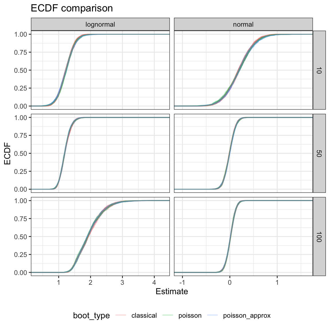

On the first sight, Poisson (and also the approximate version) look as good as the classical version. A couple of notes:

distributions get narrower (translated to ECDF: steeper) with sample size⁴;
distributions for different sample sizes have different means - remember, they are sampled from the same distribution but the observations are different;
ECDFs from smaller sample sizes look more wiggly - but on the other hand the whole distribution is wider;
bootstrap approximations work equally fine on both sample distributions.

Now let’s get from eyeballing to numbers and compare the standard errors of mean estimates for each bootstrap’s type and index.

df_plot <- df_boot %>%
  mutate(sd = map_dbl(estimates, sd, na.rm = TRUE)) %>%
  group_by(sample_size, distribution) %>%
  mutate(sd_norm = sd / mean(sd[boot_type == "classical"])) %>%
  ungroup()

ggplot(df_plot, aes(boot_type, sd_norm, fill = boot_type)) +
  geom_boxplot(alpha = 0.5, position = "dodge", show.legend = FALSE) +
  facet_grid(~sample_size ~ distribution) +
  labs(
    title = "Standard error comparison",
    x = NULL,
    y = "Normalized standard error"
  )

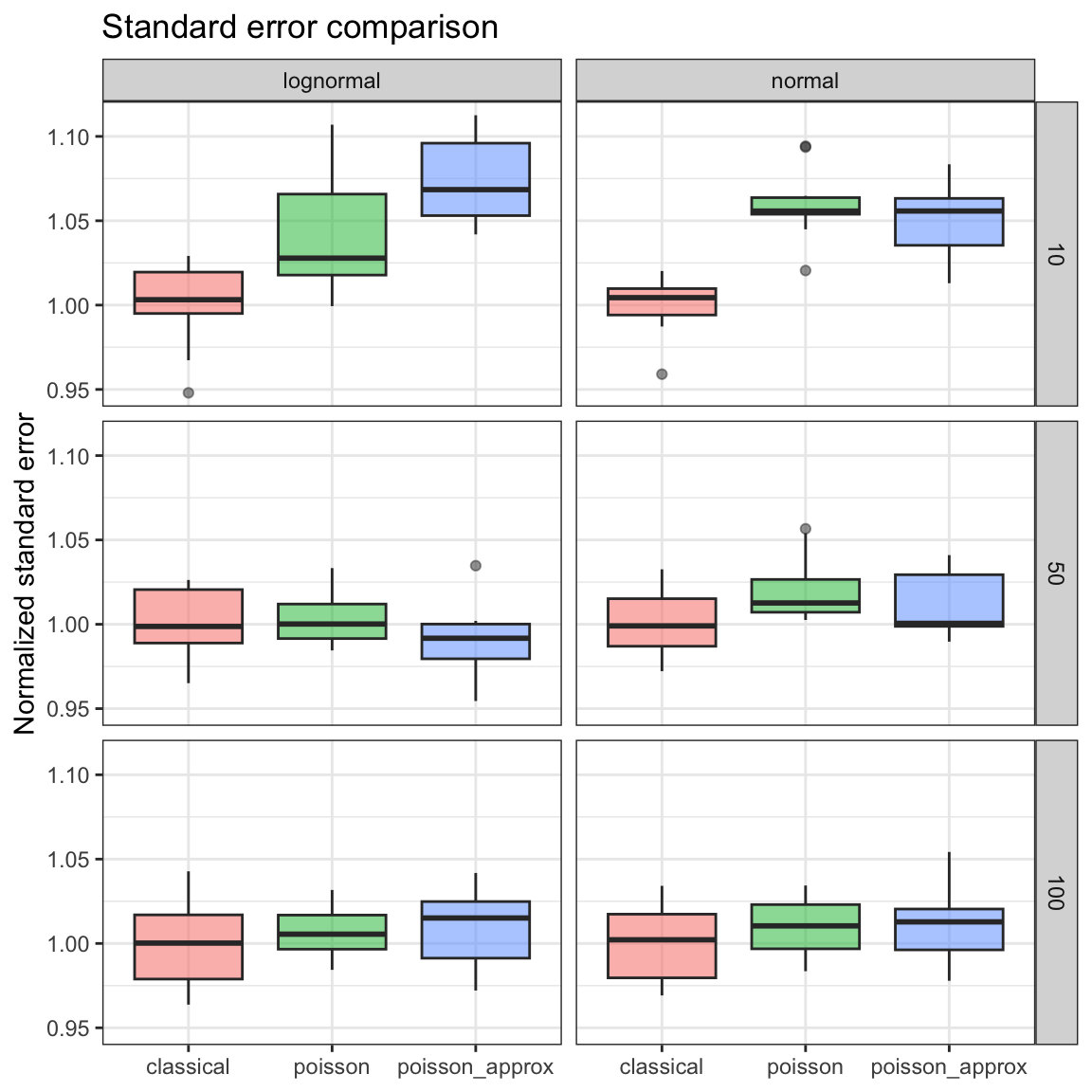
Here we can see that the 10-observation sample has around 5% higher standard error of the mean estimate. With bigger samples, the difference gets practically negligible. ⁵

I used the same procedure for the 95% confidence interval estimation and got comparable results.

Conclusion

Poisson and approximate Poisson bootstraps cause a few percentage increase in standard error (and 95% confidence interval) of the mean estimate in smaller samples (below 100). With bigger samples - no matter whether the distribution is normal or log-normal - Poisson bootstrap performs basically the same besides bringing some additional benefits, such as simplicity and possible performance improvements.

This blog is a gold mine! The level of expertise is just right that every time I learn something new and applicable.↩︎
^[An observation has \(n\) trials, each with \(\frac{1}{n}\) probability to be included in the resample.↩︎
tidyr::crossing is handy for such tasks.↩︎
Not a surprise.↩︎
If you’re interested in a formula on how this difference changes with sample size, take a look at Creating non-parametric bootstrap samples using Poisson frequencies paper from Hanley and MacGibbon.↩︎

Simpler bootstrap for big(ger) data

The classical non-parametric bootstrap

The Poisson bootstrap

Comparison

Conclusion