Employing Item Response Theory and Bayesian Multilevel Models on Strava Segments
data science
Bayesian
R
cycling
Author
Miha Gazvoda
Published
October 29, 2023
Have you ever wondered whether you’re a faster cyclist than your brother? A simple race could settle that. I learned this the hard way when I was twelve.
What about sizing up against a cyclist you bump into now and then? This is where the Strava app comes in handy. Within Strava, there’s a feature called ‘segments’ — specific stretches of road or trail, set up by users for a friendly competition. Whenever you tackle one of these segments, Strava automatically pits your time against every other user who’s taken on the same segment, giving you a leaderboard. You get insights into how you fare against others.
However, sharing a common segment is necessary for a direct comparison. But in this post, I want to demonstrate that even without sharing a segment, comparisons can still be made. Beyond that, we’ll show how to quantify a cyclist’s ability (i.e. ability is inverse of speed: time they spend on the segment). This method yields a single metric representing each cyclist’s estimated speed or ability. Using this, we can estimate a probability that one cyclist is faster than another or calculating the difference of their abilities. Welcome to the world of Item Response Theory (IRT) — the Bayesian way.
Item response theory
Traditionally, IRT models the situation in which a number of students each answer a few test questions. The model is based on parameters for the ability of the students and the difficulty of the questions. This enables to pose a set of different (but partially overlapping) questions to each student.
But how does this relate to cycling ability?
There’s a word “ability” used also in the description above. And difficulty; maybe connected with how difficult or demanding is the cycling segment? Let’s explore further.
Factors influencing cycling speed
Numerous other factors can influence how fast someone cycles. Here are a few to consider:
actual segment: how long, curvy, and steep the route is;
ability: strength and stamina of the cyclist, which is our primary focus;
effort: everyone is slower without putting in the right effort;
weather: factors like temperature, rain, and especially wind can alter riding conditions;
group riding: it’s easier due to decreased wind resistance, especially on flat.
Better (higher ability) cyclists usually ride tougher segments, in worse weather (because they also ride in winter), put in more effort. For our analysis, we’ll assume a cyclist’s ability remains consistent over time, or at least, that all our data comes from a short interval where this ability is constant.1 We will ignore factors mentioned above with the exception of segment and ability.
Data
Our data is Jeddah cycling segments leaderboard from Kaggle. When selecting relevant columns, we end up with columns for user, segment, and time spend on the segment.
library(tidyverse)library(brms)library(bayesplot)library(glue)word_to_letter <- \(x) LETTERS[as.integer(factor(x))]df <-read_csv("jeddah_strava_segments.csv") |>mutate(smt_finish_minutes = smt_finish_seconds /60,segment =word_to_letter(smt_name) ) |>select(t = smt_finish_minutes, user = user_id, segment) |>filter(t <=30) |># filter suspiciously long times mutate(across(c(user, segment), factor))head(df)
# A tibble: 6 × 3
      t user  segment
  <dbl> <fct> <fct>
1  4    1     I
2  5.88 2     I
3  6.45 3     I
4  6.48 4     I
5  6.7  5     I
6  7.17 6     I
Let’s assume time spent on a segment represents cyclist’s ability (lower time represents higher speed, and the way around).
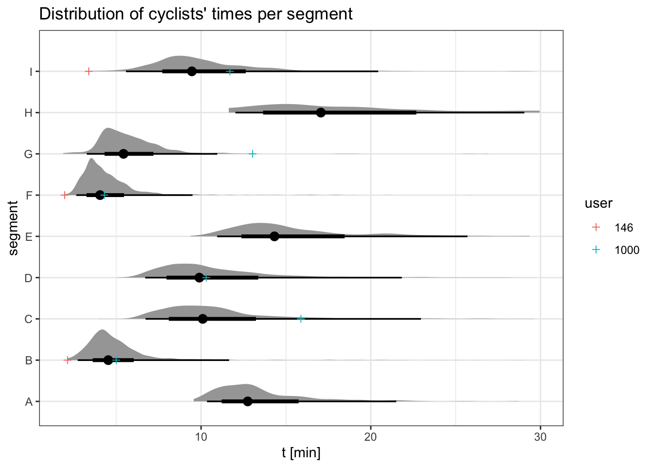
The plot below shows the distribution of times cyclists take to complete different segments. Each horizontal density represents the range of completion times for a specific segment. I’ve highlighted data points for two particular cyclists (users 146 and 1000) so we can compare their ability later on and do a sanity check.
df |>ggplot(aes(t, segment)) + tidybayes::stat_halfeye() +geom_point(aes(t, segment, color = user), shape =3, data =filter(df, user %in%c(146, 1000))) +labs(title ="Distribution of cyclists' times per segment", x ="t [min]")
Modeling
Our objective is to model the time a cyclist takes to complete a particular segment. Instead of assuming a simple additive relationship between the segment and a cyclist’s ability, it’s makes more sense to consider relative margins. A faster cyclist isn’t merely quicker by a fixed number of seconds but is faster by a certain percentage or relative margin. To achieve this, we can use log transformation on time variable (it’s the same as exponentiating and multiplying the coefficients). Here’s how the model is set up:
\(\beta_0\) is an intercept. It represents duration of an average cyclist on the average segment.
\(\beta_{1,segment[i]}\) captures the duration for \(segment_i\). (However, to actually calculate the duration, we need to take into account the intercept too.)
\(\beta_{2, user[i]}\) captures the ability of \(i\)-th cyclist.
We hypothesize that both segments and user abilities come from their own normal distributions, which are inferred from the data. This approach, known as a multilevel (or hierarchical) model2, often improves estimates, especially when dealing with limited data. For instance, such a model could provide an estimate of a cyclist’s ability even before they’ve completed a ride or if they’ve only completed a segment that no one else has tackled. While the hierarchical model adds robustness, we could establish a model without it.
We also need to set priors for \(\sigma\), \(\beta_0\), \(\sigma_{\beta_1}\), and \(\sigma_{\beta_2}\) . I’ve chosen some logical priors, though default settings would likely suffice.
priors <-c(prior(normal(2, 1), class ="Intercept"),prior(exponential(1), class ="sd"),prior(exponential(1), class ="sd", group ="segment"),prior(exponential(1), class ="sd", group ="user"))
Model implementation
To implement the previously described model using brms, we employ the formula syntax. In this setup, varying intercepts (i.e. multilevel model) are represented as (1|segment) and (1|user). However, we could opt for “fixed” intercepts by using just segment and user.
To get insights into our model, we can check its summary:
summary(model)
 Family: gaussian
  Links: mu = identity; sigma = identity
Formula: log(t) ~ (1 | segment) + (1 | user)
   Data: df (Number of observations: 7741)
  Draws: 4 chains, each with iter = 1000; warmup = 500; thin = 1;
         total post-warmup draws = 2000

Multilevel Hyperparameters:
~segment (Number of levels: 9)
              Estimate Est.Error l-95% CI u-95% CI Rhat Bulk_ESS Tail_ESS
sd(Intercept)     0.68      0.18     0.42     1.12 1.01      547      891

~user (Number of levels: 2243)
              Estimate Est.Error l-95% CI u-95% CI Rhat Bulk_ESS Tail_ESS
sd(Intercept)     0.28      0.01     0.27     0.29 1.01      441      858

Regression Coefficients:
          Estimate Est.Error l-95% CI u-95% CI Rhat Bulk_ESS Tail_ESS
Intercept     2.35      0.23     1.88     2.81 1.01      309      538

Further Distributional Parameters:
      Estimate Est.Error l-95% CI u-95% CI Rhat Bulk_ESS Tail_ESS
sigma     0.20      0.00     0.19     0.20 1.00     1656     1520

Draws were sampled using sampling(NUTS). For each parameter, Bulk_ESS
and Tail_ESS are effective sample size measures, and Rhat is the potential
scale reduction factor on split chains (at convergence, Rhat = 1).
Rhat parameters all equal one, which means the sampling was okay. The effective sample size ESS is in hundreds which is enough.
Results
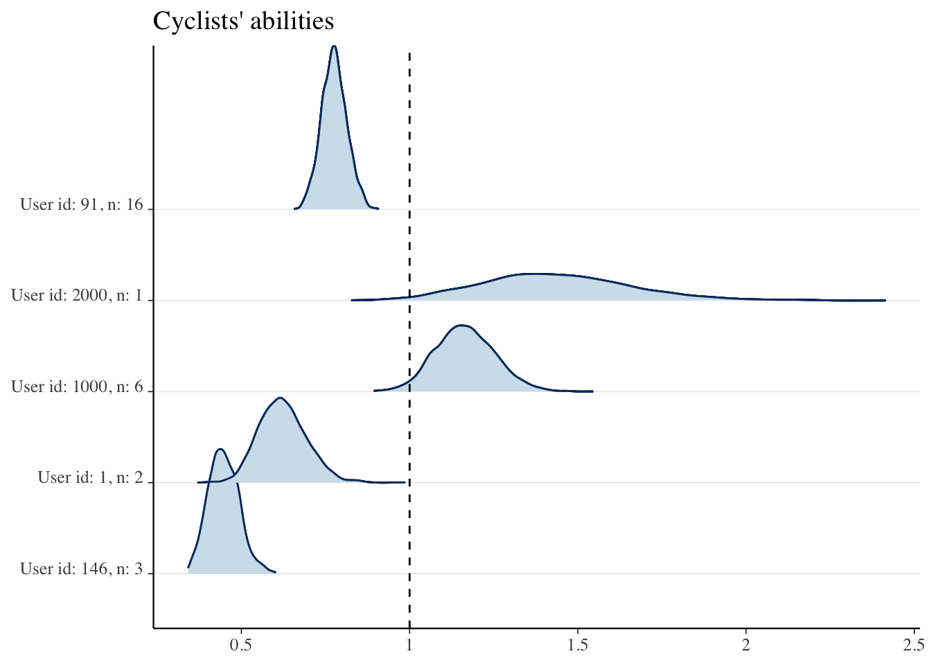
We’ll now visualize the abilities of certain cyclists. Before plotting, we’ll exponentiate the abilities for easier interpretation. For clarity: an ability of 0.5 implies that the cyclist takes only half the time an average cyclist takes on a segment (i.e., they’re twice as fast).
We can see cyclists user: 146 and user: 1000 for whom we also plotted their actual times before. user: 146 was generally performing better than the user: 1000 and also better than the average, which aligns with the estimated abilities. Users with a higher number of attempts, denoted as n, typically have less uncertainty about their ability.
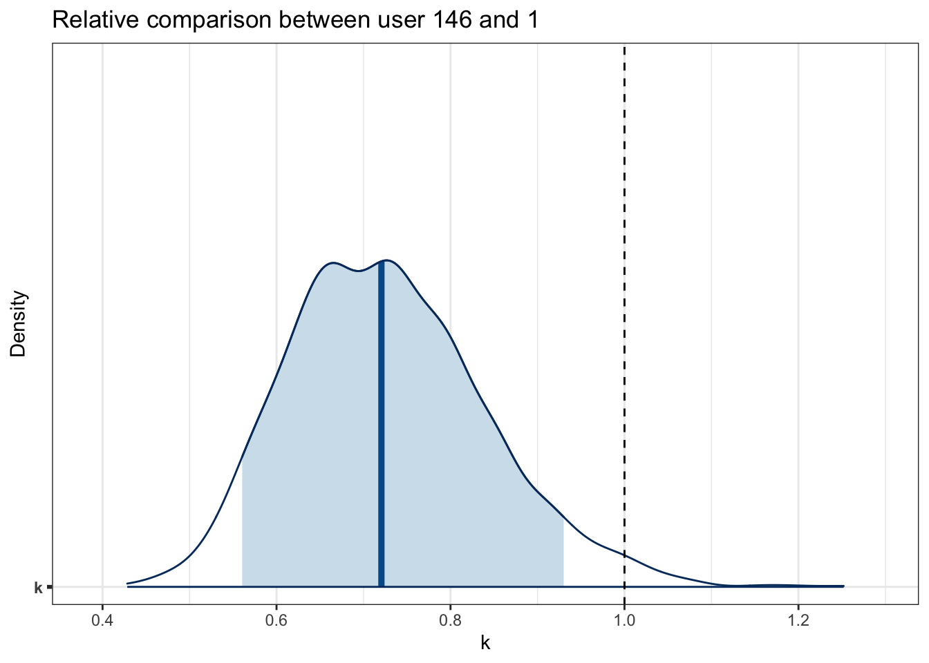
Bayesian inference lets us directly compare abilities. For instance, user: 146 is likely faster than user: 1. To understand this difference, we’ll examine the posterior samples of their abilities. By comparing these, we find that cyclist user: 146 takes around 30% less time than cyclist user: 1 on the same segment. To make a relative comparison k, we divide their exponentiated abilities.
df_diff_users <-as_draws_df( model, variable =construct_user_columns(c(146, 1))) |>mutate(k =exp(`r_user[146,Intercept]`)/exp(`r_user[1,Intercept]`))mcmc_areas(df_diff_users, pars ="k", prob =0.9) +geom_vline(xintercept =1, linetype ="dashed") +labs(title='Relative comparison between user 146 and 1', x ='k', y ='Density')
90% credible interval is excluding 1, indicating a difference in their abilities. Let’s calculate the actual probability that cyclist 146 is better than 1:
mean(df_diff_users$k <1)
[1] 0.983
This probability, while rooted in its own set of model assumptions (as every model), is both intuitive and straightforward to interpret, highlighting the power and clarity of the Bayesian approach.
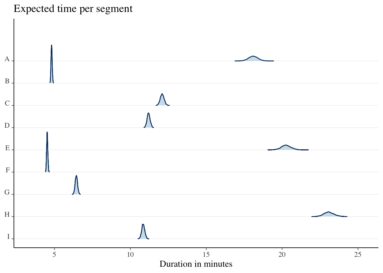
Similarly, we can plot the expected time for each segment. However, we have to sum the segment coefficient and intercept first and then exponentiate them. This way we get expected time per segment in minutes. Since we have at least a couple hundred attempts per segment, segment times have less uncertainty around them.
as_draws_df(model, variable =c("b_Intercept", "r_segment")) |>transmute(across(.cols =starts_with("r_segment"), .fns= \(x) exp(x + b_Intercept))) |>rename_with(\(x) substr(x, start=11, stop=11)) |>mcmc_areas_ridges() +labs(title='Expected time per segment', x='Duration in minutes')
To gauge how long a cyclist might take on a segment, we can just make predictions with our model and compare them with the actual values:
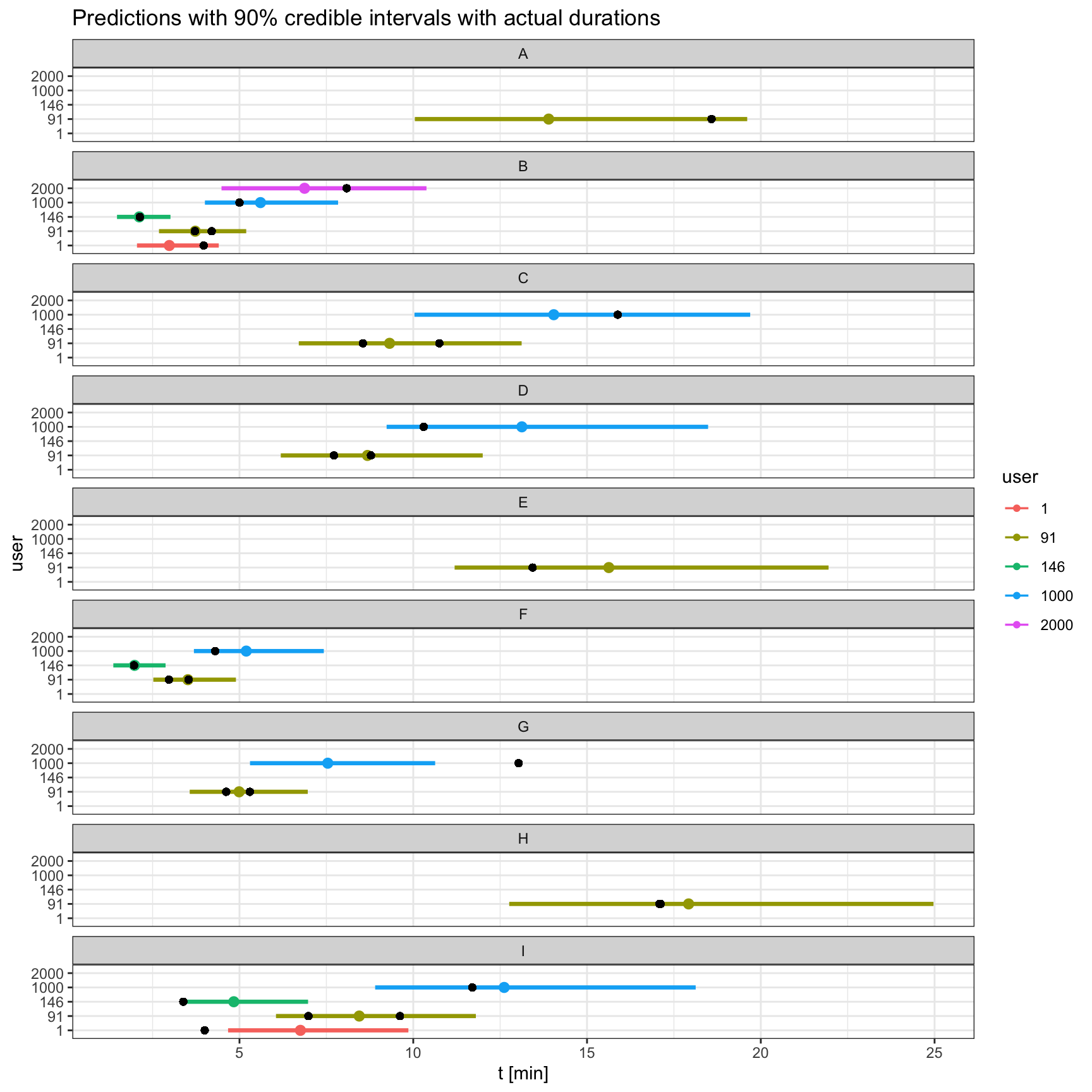
df_sampled <-filter(df, user %in% users)tidybayes::add_predicted_draws(newdata = df_sampled, object = model, value ="log_t_pred") |>mutate(t_pred =exp(log_t_pred)) |>ggplot(aes(y = user)) + ggdist::stat_pointinterval(aes(x = t_pred, color = user), .width =0.9) +geom_point(aes(x = t)) +facet_wrap(~segment, ncol =1) +labs(title="Predictions with 90% credible intervals with actual durations", x='t [min]')
Our findings align with the data. Segments B and F seem to have the shortest times. Users 1000 and 2000 take more than others to finish the segments, aligning with their lower abilities. Coverage of 90% credible intervals looks okay.
It would be even better to test our predictions on unseen data. However, the advantage is that multilevel models generally offer protection against overfitting. This can be seen from user: 2000 for whom we have only one data point. However, point estimate doesn’t precisely match the actual data point, it’s pulled towards the average ability in the population.
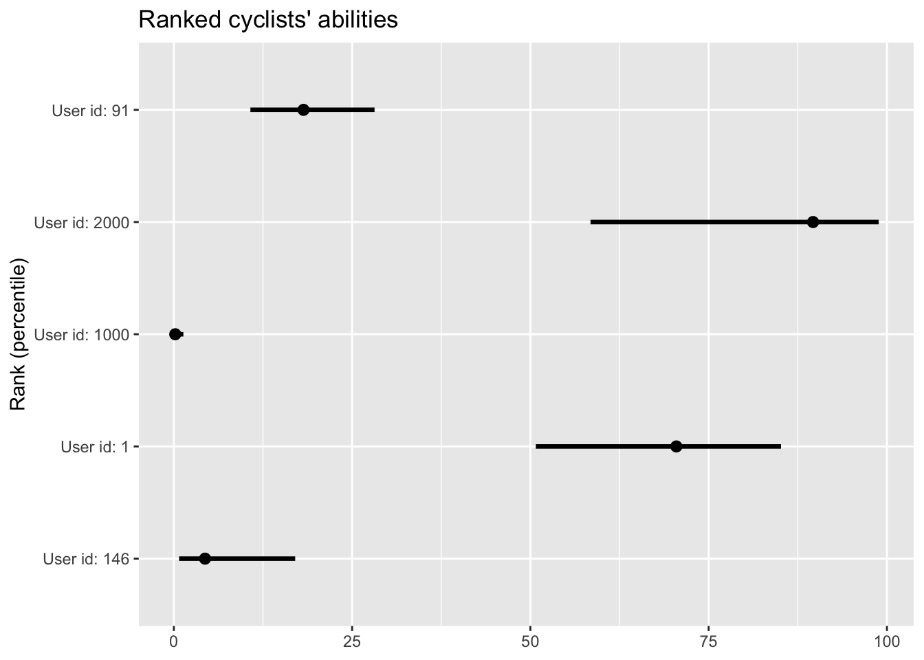
Ranking cyclists’ abilities
Ability tells you how fast you are relative to the average cyclist. However, some people might be interested in knowing how well they stand against the broader population, i.e. rank of their ability. The most direct method for this is to rank a cyclist’s posterior draws for their ability against everyone else, assigning them a percentile score between 0 and 100. This method can become time-consuming, especially with a large number of cyclists.
Luckily, multilevel structure to the rescue! This approach also provides an estimate for the standard deviation across cyclists’ abilities, termed sd_user__Intercept (or \(\sigma_{\beta_2}\) from our previous equations). With this, we can pinpoint where a particular cyclist’s ability stands in relation to the overall distribution. In technical terms, we compute the cumulative distribution function, resulting in a value between 0 and 1, which we then multiply by 100 to get the percentile rank. Importantly, since we have posterior draws for both the standard deviation and individual abilities, we can also gauge the uncertainty in our ranking estimates.
Nonetheless, some might assert that the exponentiated user abilities aren’t normally distributed, and therefore, this method may be inaccurate. While I believe this method is reasonably robust, it would be worthwhile to cross-check the results with a ranking system that conducts direct user-by-user comparisons.
Conclusion
The model offers an interesting insights into a cyclist’s performance without the need for the same location of cycling. Of course, it has a lot of room for improvements. By introducing interactions based on segment type, like vertical meters or percentage incline, we could derive specific abilities, such as climbing, descending, or sprinting. Allowing the abilities to change over time would make a model more complex, but could offer insights into a cyclist’s evolution in various performance areas.
Incorporating previously mentioned confounders, like heart rate, weather conditions, or the nature of the ride (solo vs. group), would improve the model’s precision and reduce biases.
It would be nice to have a platform where users can upload their segment times, and receive an estimate on their (overall, not only for one specific segment) ranking of ability. Whether on Strava, or some other website.
Footnotes
Of course we could also measure the change of ability over time - maybe a topic for another blog post.↩︎