Intuitive Bayesian inference

Binomial data example

I’ve struggled many times to dive into Bayesian inference. I attended a 10+ hour course (and passed it) without properly understanding what’s going on. Then, while watching the talk about linear models and using common sense¹, I came across Statistical Rethinking book and video course. ²

In the early chapters, the author focuses on presenting the topic with simple examples that can be solved without equations. And I started to understand what’s going on. Besides that, I figured out that I learn by doing - not by listening. That’s how this article (and a dashboard) was born.

Tossing

The author introduces an earth tossing example for approximating the proportion of water on the earth’s surface. You throw a globe in the air, catch it, check your index finger, write down if it’s water (1 = success) or land (0 = failure). By throwing it a lot of times you could estimate the proportion of water on earth. But how sure can you be about the estimation?

Let’s say p is a parameter of our model and presents a probability of success, i.e. probability that we will catch the earth pointing on the water which translates into the proportion of earth’s surface covered by water. Based on tossing outcomes we will estimate how likely is that each of that p could generate such data. By each p I mean all probabilities of success, from 0 to 1. They can be continuous or discrete. For example, you can focus only on each tenth quantile.

Prior

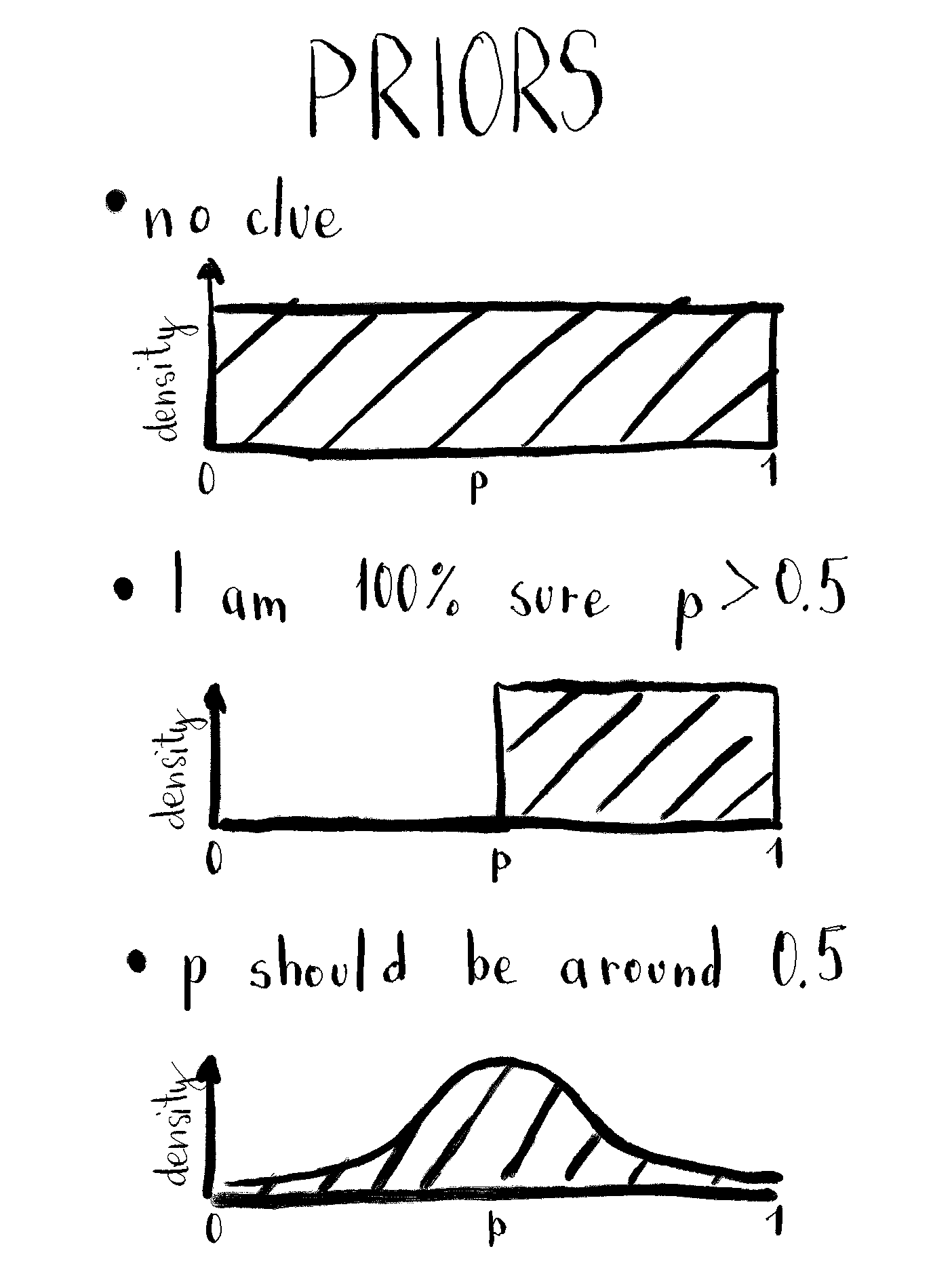
In the Bayesian world, your prior knowledge counts. If you don’t have it, also fine, but your inference won’t be as precise as it could be. In this example, prior knowledge about the parameter p is incorporated into the prior. Generally, this should be done before peeking into data.

If you don’t know anything about the proportion of water on earth you can assign the same probability to all values of parameter p. That’s called a flat prior. You usually want to avoid it.

If you know that there’s more than 50% of water on the earth’s surface, you can assign 0 prior probability to p less than 0.5.³ Or if you suspect the probability should be around 0.5, you can use normal (or beta distribution) with the mean of 0.5. It also doesn’t make sense to use too big standard deviations and cut off values below 0 and above 1.

Likelihood

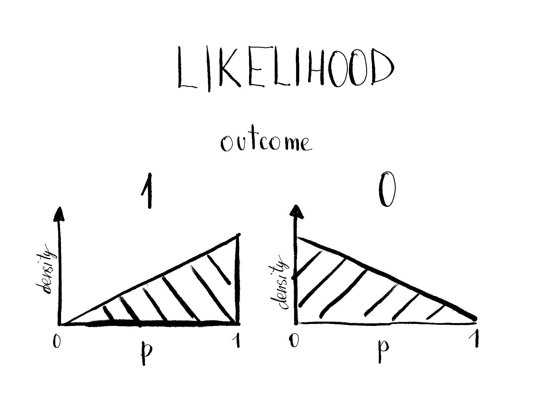
Likelihood tells you how likely a model with parameter value p probability of success would produce such outcome(s). In our example, there are only two possible outcomes, 0 and 1, for which we need to figure out the likelihoods.

What’s the probability, for example, that the model with p = 0.9 produces the outcome 1? It’s 0.9, you’re right. For 0.8, it’s 0.8, and so on. That holds for all parameter values between 0 and 1. It’s a linear relationship where higher p values have higher probability density (when outcome equals 1).

The likelihood for earth tossing outcomes. Each has to sum up to 1.

Posterior

Posterior is what we are interested in. It tells the plausibility of each parameter p given its prior probability and data. It’s proportional to a product of likelihood and prior for each value of p. To get a posterior value for p = 0.9, you just multiply the prior probability that p = 0.9 and the likelihood probability that such p generated observed data. Then you need to normalize it by dividing the posterior value by the sum of posteriors for all p. This way we get a probability (density)⁴ for each posterior p value.

Bayesian updating

But the fun doesn’t end there. Let’s say you observed multiple tosses and got outcomes 010. To get the posterior you need to calculate the likelihood for such an outcome, or - wait for it - you can do it iteratively. After each toss, each posterior can be used as a prior for the next toss. This means you can just calculate posterior as a normalized product of a prior and likelihood for each outcome. Like this:

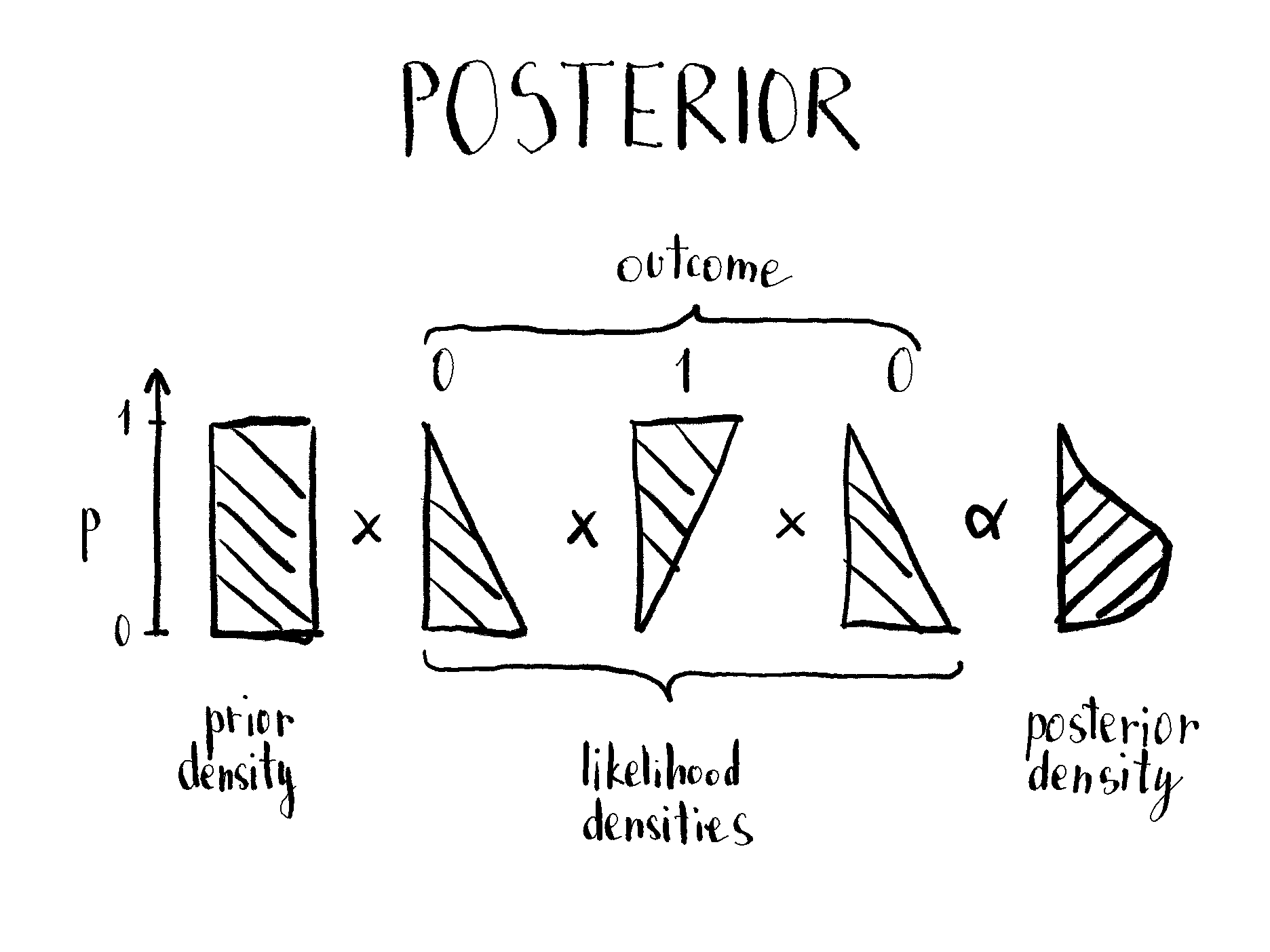
Bayesian magic. For each p you multiply prior and likelihood densities to get a proportional posterior. This can be done iteratively - for example, prior density and likelihood of the first outcome can be used as a prior for the next outcome. Note that the axes are flipped.

Simple multiplication means that posterior after 011 is the same as after 110 or 101. It also takes care that 01 is not the same as 0011. The posterior is narrower in the latter case.

Playground

I created a Shiny reactive app (see code) where you can observe Bayesian updating and get an intuition about it. It enables to play around with different priors, trial (toss) outcomes, and observe changes in posterior.

It’s (like) magic, isn’t it?

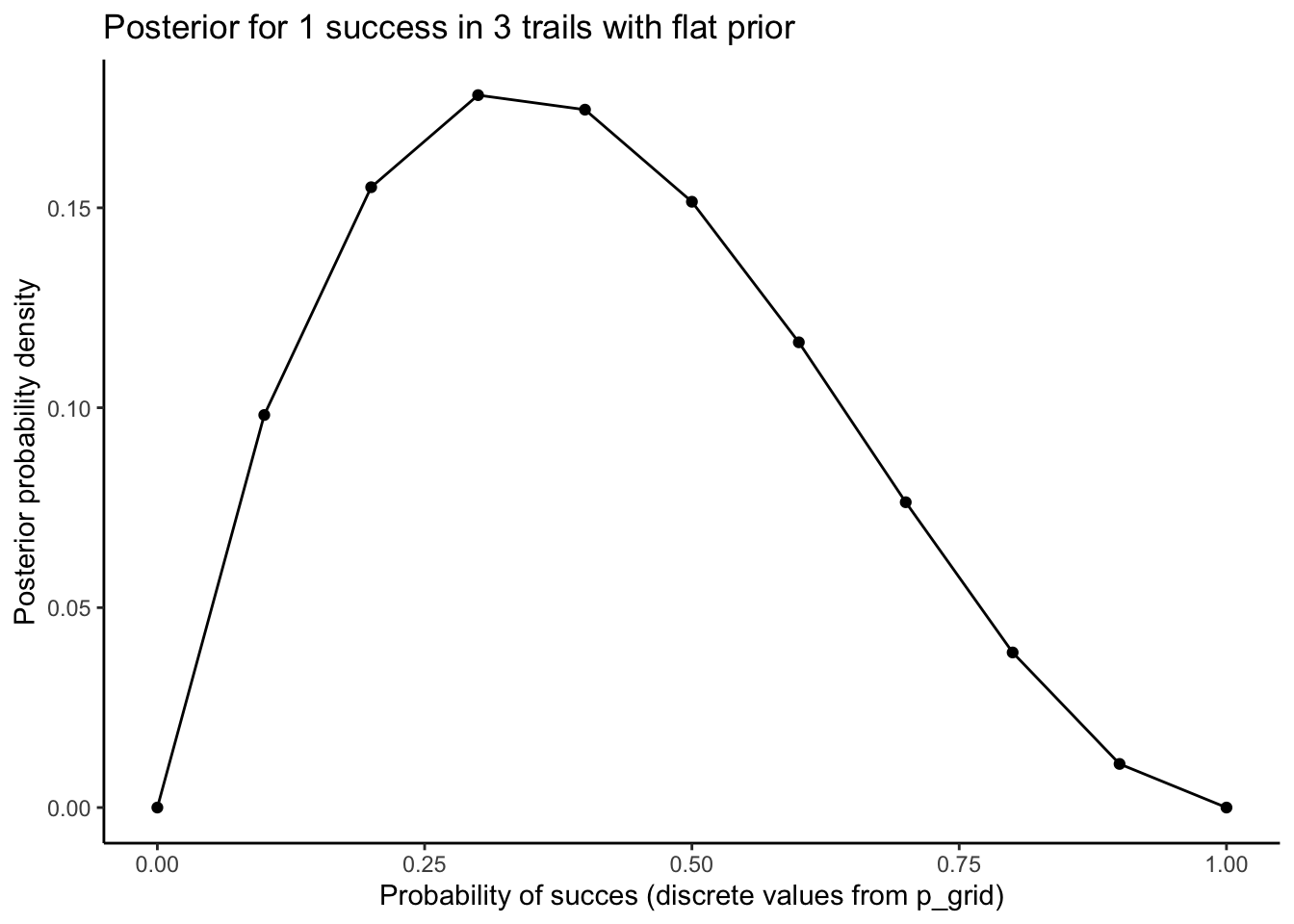
See the above example in R.

This method is called grid approximation. It means considering only a finite grid of parameter values (although the parameter is continuous).

# define number of equidistant points between 0 and 1
  n <- 11
  p_grid <- seq(from = 0, to = 1, length.out = n)
  
  # define flat prior (unstandardized)
  prior <- rep(1, n)
  
  # compute likelihood at each value in grid for 1 success in 3 trials
  likelihood <- dbinom(1, size = 3, prob = p_grid)
  
  # compute product of likelihood and prior
  unstandardized_posterior <- likelihood * prior
  
  # standardize the posterior, so it sums to 1
  posterior <- unstandardized_posterior / sum(unstandardized_posterior)
  

library(ggplot2)

ggplot(tibble::tibble(p_grid, posterior), aes(p_grid, posterior)) +
  geom_line() +
  geom_point() + 
  theme_classic() +
  labs(
    title = "Posterior for 1 success in 3 trails with flat prior",
    x = "Probability of succes (discrete values from p_grid)",
    y = "Posterior probability density"
  )

---

1. Vincent gave a couple of amazing talks on solving problems using Bayesian inference. Take a look.↩︎

2. I think they supplement each other well. If you need to pick one, go with the book. The first two chapters are available for free.↩︎

3. This means that p won’t be lower than 0.5 no matter the data.↩︎

4. We get probability because we are approximating otherwise continuous p with a grid.↩︎